4. Calculation

The kite.Calculation object contains the information required to calculate desired quantities, i.e. the target functions. Key parameters of the calculation are included here, such as the Chebyshev expansion order and number of disorder realizations. These are used by KITEx to calculate the spectral coefficients. Subsequently, at the post-processing stage, KITE-tools can be used, e.g. to reconstruct the full energy dependence of the desired target function (see Workflow). The parameters given in the Examples are optimized for relatively small systems and are therefore ideal to run KITE with a standard desktop computer or laptop.

The target functions currently available are:

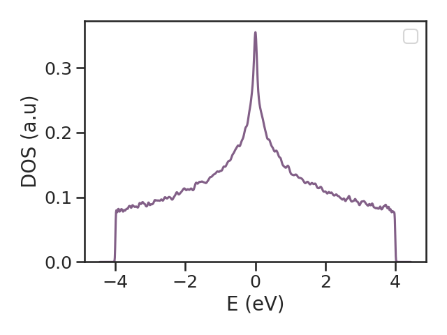
• dos

  Calculates the average density of states (DOS) as a function of energy.

• ldos

  Calculates the local density of states (LDOS) as a function of energy (for a set of lattice positions).

• arpes

  Calculates the one-particle spectral function of relevance to ARPES.

• gaussian_wave_packet

  Simulates the propagation of a gaussian wave-packet.

• conductivity_dc

  Calculates a given component of the DC conductivity tensor.

• conductivity_optical

  Calculates a given component of the linear optical conductivity tensor.

• conductivity_optical_nonlinear

  Calculates a given component of the 2nd-order nonlinear optical conductivity tensor.

• singleshot_conductivity_dc

  Calculates the longitudinal DC conductivity for a set of Fermi energies (uses the \(\propto\mathcal{O}(N)\) single-shot method).

The table below shows to which level the KITE target functions have been implemented and tested at the time of writing (May, 2025). Note that the non-linear optical conductivity functionality is currently restricted to 2D systems.

Method	2D	3D
dos
ldos
arpes
gaussian_wave_packet
conductivity_dc
conductivity_optical
conductivity_optical_nonlinear
magnetic_field
singleshot_conductivity_dc

- Checked and extensively used

- Implemented and checked

- Not yet implemented

All target functions require the following parameter:

• num_moments

  Defines the order of Chebyshev expansions and hence the effective energy resolution of the calculation; see Documentation.

Other common parameters are:

• num_random

  Defines the number of random vectors used in the stochastic trace evaluation.

• num_disorder

  Defines the number of disorder realizations (and automatically specifies the boundary twist angles if the "random" boundary mode is chosen; see Settings).

Some functions also require the following parameters:

• direction

  Specifies the component of the linear (longitudinal: ('xx', 'yy', 'zz'), transversal: ('xy', 'yx', 'xz', 'yz')) or the nonlinear conductivity tensor (e.g., 'xyx' or 'xxz') to be calculated.

• temperature (can be modified at post-processing level)

  Temperature of the Fermi-Dirac distribution used to evaluate optical and DC conductivities. temperature specifies the quantity \(k_B T\), which has units of energy. For example, if the hoppings are given in eV, temperature must be given in eV.

• num_points (can be modified at post-processing level)

  Number of energy points used by the post-processing tool to output the dos and other target functions.

• energy

  Selected values of Fermi energy at which we want to calculate the singleshot_conductivity_dc.

• eta

  Imaginary constant (scalar self energy) in the denominator of the Green's function required for lattice calculations of finite-size systems, i.e. an energy resolution (can also be seen as a controlled broadening or inelastic energy scale). For technical details, see Documentation.

The calculation is structured in the following way:

calculation = kite.Calculation(configuration)
calculation.dos(
    num_points=1000,
    num_random=10,
    num_disorder=1,
    num_moments=512
)
calculation.conductivity_optical(
    num_points=1000,
    num_random=1,
    num_disorder=1,
    num_moments=512,
    direction='xx'
)
calculation.conductivity_dc(
    num_points=1000,
    num_moments=256,
    num_random=1,
    num_disorder=1,
    direction='xy',
    temperature=1
)
calculation.singleshot_conductivity_dc(
    energy=[(n / 100.0 - 0.5) * 2 for n in range(101)],
    num_moments=256,
    num_random=1,
    num_disorder=1,
    direction='xx',
    eta=0.02
)
calculation.conductivity_optical_nonlinear(
    num_points=1000,
    num_moments=256,
    num_random=1,
    num_disorder=1,
    direction='xxx',
    temperature=1.0,
    special=1
)

Note

The user can decide what functions are used in a calculation. However, it is not possible to configure the same function twice in the same configuration file.

When these objects are defined, we can set up the I/O instructions for KITEx using the kite.config_system function:

kite.config_system(lattice, configuration, calculation, filename='test.h5')

Export the KITE model to the I/O HDF file, by running

python3 script_name_here.py

Running a Calculation

To run the code and to post-process it, run from the kite/-directory

./build/KITEx test.h5
./build/KITE-tools test.h5

KITE-tools output

The output of KITE-tools is dependent on the target function specified by the user. Each specific case is described in the API. This output is generally a "*.dat"-file where the various columns of data contain the required target functions.

Visualizing the Output Data

After calculating and post-processing the target functions, we can plot the resulting data with the following script:

data=np.loadtxt('dos.dat')

plt.plot(data[:,0], data[:,1])
plt.xlabel('E (eV)')
plt.ylabel('DOS (a.u)')

A more streamlined approach would be to use a Bash script, for example:

#!/bin/bash

file_out=example1                 # name of python script that exports the HDF5-file
file_in=example1                  # name of the exported HDF5-file

python ${file_out}.py             # make a model
./build/KITEx ${file_in}.h5       # run Kite

./build/KITE-tools ${file_in}.h5  # run the post-processing steps
python plot_dos.py                # display the data