Skip to content

Graphene

The TB-model for Graphene

The electronic structure of graphene is well-described by a simple tight-binding model that only uses one \(p_z\) orbital in a hexagonal unit cell with two equivalent carbon atoms. These atoms are located on the different sublattices, A and B, and don't have an on-site energy term.

Although this model is relatively simple, it is used often within the literature. The example below uses graphene to show how to construct a lattice with sublattices and perform a basic calculation using KITE. The script for this example can be found here.
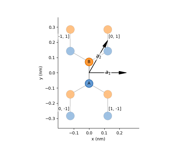
Lattice

We start by building the pb.lattice for graphene:

  • Define the parameter (\(t\) in eV)
  • Define the vectors of the unit-cell (\(\vec a_1\) and \(\vec a_2\) in units of \(a\), length of the unit-cell)
  • Create a pb.lattice-object
  • Define the on-site energies
  • Define the hopping parameters
    • 1 normal hopping within the unit cell
    • 2 rotated hopping \(\pm 2 \pi/3\) to neighbouring cells
  • Return the pb.lattice-object to be used by KITE
def graphene_lattice(onsite=(0, 0)):
    """Return lattice specification for a honeycomb lattice with nearest neighbor hoppings"""

    # parameters
    a = 0.24595  # [nm] unit cell length
    a_cc = 0.142  # [nm] carbon-carbon distance
    t = 2.8  # eV

    # define lattice vectors
    a1 = a * np.array([1, 0])
    a2 = a * np.array([1 / 2, 1 / 2 * np.sqrt(3)])

    # create a lattice with 2 primitive vectors
    lat = pb.Lattice(a1=a1, a2=a2)

    # add sublattices
    lat.add_sublattices(
        # name, position, and onsite potential
        ('A', [0, -a_cc/2], onsite[0]),
        ('B', [0,  a_cc/2], onsite[1])
    )

    # Add hoppings
    lat.add_hoppings(
        # inside the main cell, between which atoms, and the value
        ([0, 0], 'A', 'B', -t),
        # between neighboring cells, between which atoms, and the value
        ([1, -1], 'A', 'B', -t),
        ([0, -1], 'A', 'B', -t)
    )
    return lat

We can visualize this lattice using the following code:
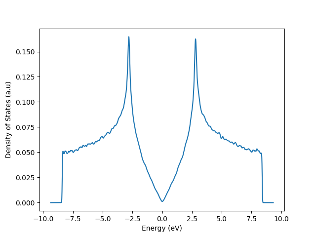
1
2
3
lat = graphene_lattice()
lat.plot()
plt.show()
A visualization for the defined lattice of graphene.

KITEx calculation

Settings and calculation

We can make the kite.Calculation object

configuration = kite.Configuration(
  divisions=[64, 64],
  length=[512, 512],
  boundaries=["periodic", "periodic"],
  is_complex=False,
  precision=1
)
calculation = kite.Calculation(configuration)
calculation.dos(
  num_points=4000,
  num_moments=256,
  num_random=256,
  num_disorder=1
)
Set up the kite.config_system as detailed in Sec. Calculation and export the KITE model running
python3 script_name_here.py
which then creates the necessary HDF file. Next, run the KITEx program and the KITE-tools.

Visualization

1
2
3
4
5
6
import numpy as np
import matplotlib.pyplot as plt

data = np.loadtxt('dos.dat')
plt.plot(data[:,0], data[:,1])
plt.show()
The DOS for graphene.