Haldane

The Haldane model¶

The Haldane Hamiltonian is a single-orbital tight-binding model on a honeycomb lattice with a sublattice-staggered on-site potential (orbital mass). Complex hoppings between next-nearest-neighbor sites produce a staggered magnetic field configuration with vanishing total flux through the unit cell ¹.

This model describes a Chern insulator (or a quantum anomalous Hall insulator) because it hosts an integer quantum Hall effect in the absence of any applied external magnetic fields. This characteristic makes Haldane model ideal for illustrating another capability of KITE: the calculation of transverse conductivities reflecting the quantum geometry of wavefunctions ² ³.

Let us use KITE to compute the dc conductivity tensor of the Haldane model. The full script for this example can be found here.

Lattice¶

Let us begin with the definition of the Hamiltonian for the case of purely imaginary next-nearest-neighbor hoppings:

def haldane(onsite=(0, 0), t=1):
    """Return lattice specification for Haldane model"""

    # parameters
    a = 0.24595  # [nm] unit cell length
    a_cc = 0.142  # [nm] carbon-carbon distance
    t2 = t/10

    # define lattice vectors
    a1 = a * np.array([1, 0])
    a2 = a * np.array([1 / 2, 1 / 2 * np.sqrt(3)])

    # create a lattice with 2 primitive vectors
    lat = pb.Lattice(a1=a1, a2=a2)

    # add sublattices
    lat.add_sublattices(
        # name, position, and onsite potential
        ('A', [0, -a_cc/2], onsite[0]),
        ('B', [0,  a_cc/2], onsite[1])
    )

    # Add hoppings
    lat.add_hoppings(
        # inside the main cell, between which atoms, and the value
        ([0,  0], 'A', 'B', -t),
        # between neighboring cells, between which atoms, and the value
        ([1, -1], 'A', 'B', -t),
        ([0, -1], 'A', 'B', -t),
        ([1, 0], 'A', 'A', -t2 * 1j),
        ([0, -1], 'A', 'A', -t2 * 1j),
        ([-1, 1], 'A', 'A', -t2 * 1j),
        ([1, 0], 'B', 'B', -t2 * -1j),
        ([0, -1], 'B', 'B', -t2 * -1j),
        ([-1, 1], 'B', 'B', -t2 * -1j)
    )
    return lat

KITEx part¶

Settings¶

The following explains the steps to calculate the Hall conductivity. The first step is to define kite.configuration, as explained in Settings. For example,

configuration = kite.Configuration(
divisions=[2, 2],
length=[128, 128],
boundaries=['periodic', 'periodic'],
is_complex=True,
precision=0,
spectrum_range=[-10, 10]
)

Then, we can set kite.calculation. We note that the the post-processing tool uses the energy spectrum limits in the HDF file ([-10,10] in the example above) to perform the integration over the energy of occupied states.

calculation.conductivity_dc(num_points=1000,
                            num_moments=256,
                            num_random=50,
                            num_disorder=1,
                            direction='xy',
                            temperature=0.05)

Disorder¶

We can include different types of disorder. For simplicity, we consider on-site uniform disorder distribution with width of 0.4 and zero average on-site energy (Anderson disorder):

disorder = kite.Disorder(lattice)
disorder.add_disorder('A', 'Uniform', +0.0, 0.4)
disorder.add_disorder('B', 'Uniform', +0.0, 0.4)

Calculation and post-processing¶

Export the KITE model to an HDF file (see Sec. Calculation) and run the KITEx program.

This is a full spectral calculation where KITEx calculates the coefficients of the Chebyshev expansion, and KITE-tools uses those moments to retrieve the transverse conductivity over the full energy range. Both temperature and num_points are parameters used by KITE-tools, and it is possible to modify them without running KITEx again. This type of calculation typically requires more RAM memory than DOS or single-shot DC conductivity, which imposes limitations to the sizes of the systems (that can still reach large scales with available memory). This has implications for the stochastic trace evaluation (STE) done by KITE, whose relative error typically scales with \(1/\sqrt{N_R D}\) (here, \(N_R\) is the number of random vectors and \(D\) is the total number of sites). The STE errors can thus be significant, especially at large Chebyshev orders (required to achieve fine energy resolutions). More generally, the relative error of the STE also depends on the lattice model, type of disorder and the calculated quantities. Transverse conductivities have strong fluctuations outside of the topological gap. This tutorial aims to illustrate this issue.

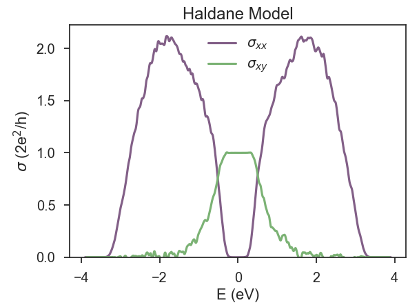
Fig. 1 below shows the longitudinal and transverse conductivity for a small lattice of Haldane model in a calculation that took a few minutes on a laptop. KITEx captures the anomalous quantum Hall plateau extremely well, with a relative error of less than 0.1%. But it is also clear that the transverse conductivity presents significantly more fluctuations outside the plateau than the longitudinal conductivity, and we already considered 50 random vectors. A finer energy resolution can be obtained by running the simulation for larger systems and/or increasing the number of random vectors used in the STE (see below).

This figure can be reproduced using KITE-tools while specifying some additional parameters (refer to the post-processing tools documentation if you need more details). To this end, run the following line

./build/KITE-tools haldane.h5 --CondDC -F -4 4 1000

which calculates the xy conductivity of the system specified above for 1000 equidistant Fermi energies in the range [-4, 4]. The result can be plotted by using the brief Python script below. (The computation and visualization of the longitudinal conductivity follows identical steps.)

Visualisation¶

import numpy as np
import matplotlib.pyplot as plt

data = np.loadtxt('condDC.dat')
plt.plot(data[:,0], data[:,1])
plt.show()

We now focus on strategies to decrease the fluctuations. Depending on the computational resources, one possibility is increasing the system size. It is also possible to increase the number of random vectors. This is illustrated in Fig. 2.

Finally, there are other ways of damping the STE fluctuations, e.g. via a simple thermal averaging effect (temperature) or the use of uncorrelated disorder. The use of such strategies depend on the goals of the numerical calculation. In the present case, where we primarily wanted to see the quantum anomalous Hall plateau, we can simply consider a moderate Anderson disorder and work with intermediate temperatures.

Example

Get more familiar with KITE: tweak the full script for this calculation and play with variations of system size, number of random vectors, disorder and temperature.

F. D. M. Haldane, Phys. Rev. Lett. 61, 2015 (1988) ↩
J. H. García, L. Covaci, and T. G. Rappoport, Phys. Rev. Lett. 114, 116602 (2015) (Supplementary material) ↩
S. G. de Castro, J. M. V. P. Lopes, A. Ferreira, and D. A. Bahamon, Phys. Rev. Lett. 132, 076302 (2024) ↩