Phosphorene

Phosphorene

This is a small tutorial to illustrate the use of KITE to investigate materials with anisotropic electrical conductivity. To this end, we consider a simplified tight-binding model for single layer phosphorene ¹. Even though this model is very simple, it captures the anisotropic band structure of phosphorene, which is Dirac-like in one direction and Schrödinger-like in the other direction. This behaviour results in highly anisotropic transport properties ².

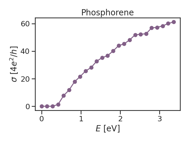
Here, we calculate the longitudinal conductivity (singleshot_conductivity_dc) via the efficient single-shot CPGF algorithm ³ in the vicinity of the band gap. This is a fast numerical calculation that is set to easily run on a standard laptop, which qualitatively reproduces the expected anisotropic conductivity along xx and yy directions.

Here, we highlight parts of the Python script. The full script can be retrieved from KITE's Github repository.

Lattice

After the imports that are necessary for KITE, we define the lattice with Pybinding:

from numpy import cos, sin, pi

def monolayer_4band(num_hoppings=4):
    """Monolayer phosphorene lattice using the four-band model

    Parameters
    ----------
    num_hoppings : int
    Number of hopping terms to consider: from t2 to t5.
    """
    a = 0.222  # nm
    ax = 0.438  # nm
    ay = 0.332  # nm
    theta = 96.79 * (pi / 180)
    phi = 103.69 * (pi / 180)

    lat = pb.Lattice(a1=[ax, 0], a2=[0, ay])

    h = a * sin(phi - pi / 2)
    s = 0.5 * ax - a * cos(theta / 2)
    lat.add_sublattices(('A', [-s/2,        -ay/2, h], 0),
                       ('B', [ s/2,        -ay/2, 0], 0),
                       ('C', [-s/2 + ax/2,     0, 0], 0),
                       ('D', [ s/2 + ax/2,     0, h], 0))

    lat.register_hopping_energies({'t1': -1.22, 't2': 3.665, 't3': -0.205,
                               't4': -0.105, 't5': -0.055})

    if num_hoppings < 2:
        raise RuntimeError("t1 and t2 must be included")
    elif num_hoppings > 5:
        raise RuntimeError("t5 is the last one")

    if num_hoppings >= 2:
        lat.add_hoppings(([-1,  0], 'A', 'D', 't1'),
                         ([-1, -1], 'A', 'D', 't1'),
                         ([ 0,  0], 'B', 'C', 't1'),
                         ([ 0, -1], 'B', 'C', 't1'))
         lat.add_hoppings(([ 0,  0], 'A', 'B', 't2'),
                         ([ 0,  0], 'C', 'D', 't2'))
    if num_hoppings >= 3:
         lat.add_hoppings(([ 0,  0], 'A', 'D', 't3'),
                          ([ 0, -1], 'A', 'D', 't3'),
                          ([ 1,  1], 'C', 'B', 't3'),
                          ([ 1,  0], 'C', 'B', 't3'))
    if num_hoppings >= 4:
        lat.add_hoppings(([ 0,  0], 'A', 'C', 't4'),
                         ([ 0, -1], 'A', 'C', 't4'),
                         ([-1,  0], 'A', 'C', 't4'),
                         ([-1, -1], 'A', 'C', 't4'),
                         ([ 0,  0], 'B', 'D', 't4'),
                         ([ 0, -1], 'B', 'D', 't4'),
                         ([-1,  0], 'B', 'D', 't4'),
                         ([-1, -1], 'B', 'D', 't4'))
    if num_hoppings >= 5:
         lat.add_hoppings(([-1,  0], 'A', 'B', 't5'),
                         ([-1,  0], 'C', 'D', 't5'))

    lat.min_neighbors = 2
    return lat

Note that the lattice model given above can be used with different numbers of hoppings. The user can decide the number that is used in the calculation when defining the lattice:

lattice=monolayer_4band(num_hoppings=4)

KITEx part

Settings

To use the large-scale single-shot algorithm for direct evaluation of zero-temperature DC conductivities, the resolvent operator requires a nonzero broadening (resolution) parameter eta, which is given in the specified units (eV in the example above). As this type of calculation is energy-dependent, it is also necessary to provide a list of desired energy points to the calculation object. In the single-shot calculations, the computational time scales linearly with the energy points. For this example, we consider a small number of points and the energy range is set in the vicinity of the band gap.

The number of points and the list of energy points can be created when calling the calculation, as illustrated here:

calculation = kite.Calculation(configuration)
npoints = 25
epoints = [(1.0 / npoints * i) * 3.5  for i in range(npoints)]
calculation.singleshot_conductivity_dc(epoints,
                                       num_moments=512,
                                       num_random=5,
                                       num_disorder=1,
                                       direction='xx',
                                       eta=0.02)

Now it is time to save the configuration in a hdf file:

kite.config_system(lattice, configuration, calculation, filename='phxx.h5')

Export the KITE model to an HDF file:

python3 script_name_here.py

Calculation

Run the KITEx program.

Visualization

After running KITEx, no post-processing is required for the single-shot conductivity calculation. The result can be extracted and plotted with the following script:

import h5py
import matplotlib.pyplot as plt

file_name = 'phxx.h5'

num_points = 25
energy = [(1.0 / num_points * i) * 3.5 for i in range(num_points)]

file_input = h5py.File(file_name, 'r+')
single_shot = file_input['Calculation']['singleshot_conductivity_dc']['SingleShot']
cond = single_shot[:, 3]

plt.plot(energy, cond, 'o-')
plt.xlabel('$E$ [eV]')
plt.ylabel(r'$\sigma$ [$4e^2 / h$]')
plt.title('Phosphorene')

plt.tight_layout()
plt.show()

Alternatively, the single-shot post-processing python tool in the tools directory can be used to produce the data in a more streamlined fashion (see Sec. Post-Processing).

Figure 1: Longitudinal DC conductivity as a function of Fermi energy for a small system computed with the single-shot CPGF algorithm.

It is not possible to request the same type of calculation (target function) in a single call. In this case, we want to calculate the conductivity in xx and yy directions where the type of the calculation is the same, which means we need another HDF file for yy conductivity.

Let's repeat the procedure for another direction (one may also use the streamlined approach of the example on the KITE repository):

    calculation.singleshot_conductivity_dc(epoints,
                                           num_moments=512,
                                           num_random=5,
                                           num_disorder=1,
                                           direction='xx',
                                           eta=0.02)
    kite.config_system(lattice, configuration, calculation, filename='phyy.h5')

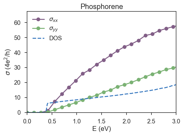
The result of this fast calculation can be seen in Fig. 2 below, for lx=ly=512. To gain confidence with using KITE, we suggest modifying parameters like eta and num_random.

Figure 2: Longitudinal and transverse components of the DC conductivity tensor and the DoS as a function of Fermi energy.

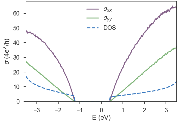
In Fig. 3, we repeat the calculation for 300 energy points and 10 random vectors with a large energy window.

Figure 2: Similar to Fig. 1, but over a larger energy window and with lower statistical fluctuations.

---

1. Alexander N. Rudenko, Mikhail I. Katsnelson, Phys. Rev. B 89, 201408 (2014). ↩

2. H. Liu, A. T. Neal, Z. Zhu, X. Xu , D. Tomanek and P. D. Ye, ACS Nano 8, 4033 (2014) ↩

3. A. Ferreira and E. R. Mucciolo, Phys. Rev. Lett. 115, 106601 (2015). ↩