2. Lattice
The aim of the current section is to help us gain familiarity with the lattice model of KITE.
Thus, we begin by constructing a periodic pb.Lattice using Pybinding
and calculating its band structure using pb.Solver (also from Pybinding).
In the following sections, we will learn how to use KITEx to significantly scale up the simulations and introduce modifications to the lattice model.
For efficiency, the default options of KITE's core code (KITEx) assume that the lattice model has a certain degree of interconnectivity or hopping range.
Specifically, the default is that the tight-binding Hamiltonian has non-zero matrix elements between orbitals that belong to unit cells
that are separated by at most 2 lattice spacings along a given direction (for example, in a simple single-orbital 1D chain this would allow defining models
with up to second-nearest neighbors). To relax this constraint and thus be able to simulate more complex lattice models, users must adjust the NGHOSTS parameter in kite/Src/Generic.hpp and recompile KITEx, otherwise an error message is output and the KITE program exits.
Info
If you are familiar with Pybinding, you can go directly to the next tutorial page.
Note
The python script that generates KITE's input file requires a few packages that can be included with the following aliases
Constructing a pb.Lattice
The pb.Lattice class from Pybinding carries the information about the TB model.
This includes:
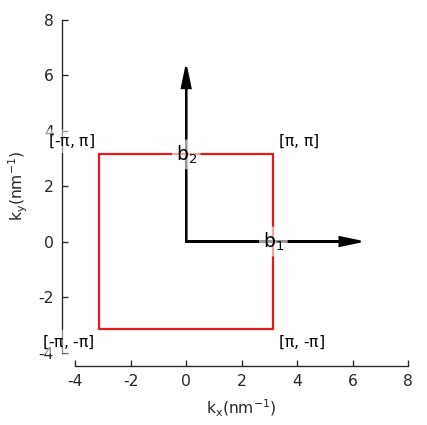
Pybinding also provides additional functionalities based on the above real-space information. For example, it can prove the reciprocal vectors and the Brillouin zone.
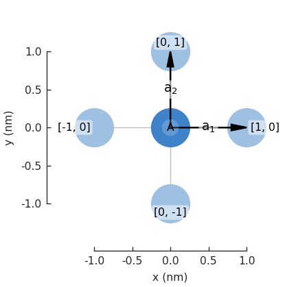
Defining the unit cell
As a simple example, let us construct a square lattice with a single orbital per unit cell. The following syntax can be used to define the primitive lattice vectors:
Adding lattice sites
We can then add the desired lattice sites/orbitals inside the unit cell (the same syntax can be used to add different orbitals in a given position or more sites in different sublattices):
Adding hoppings
By default, the main unit cell has the index [n1,n2] = [0, 0].
The hoppings between neighboring sites can be added with the simple syntax:
Here, the relative indices n1,n2 represent the number of integer steps - in units of the primitive lattice vectors - needed to reach a neighboring cell starting from the origin.
If the lattice has more than one sublattice, the hoppings can connect sites in the same unit cell.
Note
When adding the hopping (n, m) between sites n and m,
the conjugate hopping term (m, n) is added automatically. Pybinding does not allow the user to add them manually.
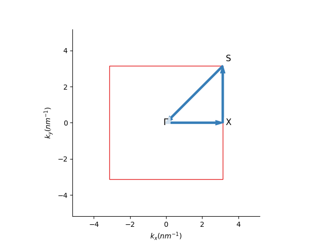
Visualization
Now we can plot the pb.lattice and visualize the Brillouin zone:
Examples
For a crystal with two atoms per unit cell, look in the Examples section. For other examples and pre-defined lattices, consult the Pybinding documentation.
Using Pybinding's solver
Pybinding has built-in solvers for
To use any of these solvers, we need to first construct a model.
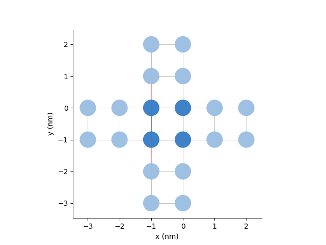
Building a pb.Model
The pb.Model class contains all the information of the structure we want to use in our calculation.
This structure can be significantly larger than the unit cell (stored in the pb.Lattice class). It can also have specific geometries and other possible modifications of the original lattice.
Here, we will double the unit cell in both directions in the pb.Model and add periodic boundary conditions:
pb.Model with
Defining a pb.Solver
The pb.Solver class takes a pb.Model class as input and prepares the system to perform a numerical calculation. We will use the LAPACK solver:
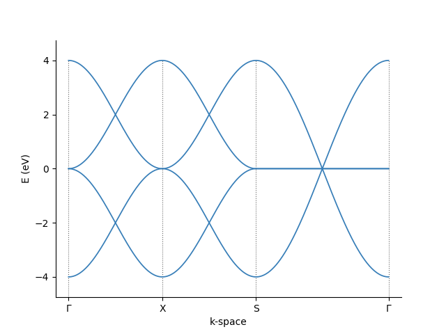
Band structure calculation
As an example, the band structure is calculated using the pb.Solver defined above.
First, for a two-dimensional plot, we define a path in the reciprocal space that connects the high symmetry points. Using the pb.Lattice built-in
method, the high-symmetry points for the corners of a path can be found easily:
We can then pass these corners to the pb.Solver and visualize the result
For more info about Pybinding's capabilities, look at its tutorial or API guide.
Summary of the code from this section