Optical Conductivity
Gaussian disorder
KITE can also calculate the optical conductivity of a given tight-binding model for any desired chemical potential/temperature. To illustrate this capability, here we calculate the optical conductivity of disordered graphene that can be compared qualitatively with previous results1. The full script can be found here.
Lattice
Instead of manually defining the lattice, we can use of one the pre-defined lattices from Pybinding:
KITEx part
Disorder
To illustrate a different type of disorder, we add random on-site energies that follow a Gaussian distribution:
    disorder = kite.Disorder(lattice)
    disorder.add_disorder('B', 'Gaussian', 0.0, 1.5)
    disorder.add_disorder('A', 'Gaussian', 0.0, 1.5)
where we define the type of statistical distribution, the sublattices where they are located, the mean value of the distribution and its width (in eV here).
Settings and calculation
After configuring the system, as presented in the Getting Started tutorial, it is time to set up the calculation:
    calculation = kite.Calculation(configuration)
    calculation.conductivity_optical(num_points=1000, num_disorder=1,
                     num_random=20, num_moments=512, direction='xx')
The transverse optical conductivity (xy,xz, etc.) can also be calculated, which can be quite interesting in systems that also present transverse responses (e.g. due to a nontrivial band topology) 3.
However, in this example we focus exclusively on the longitudinal optical conductivity.
The other quantities that can be set in the Python script are the same as for the calculation of the density of states: number of energy points used in KITE-tools, Chebyshev moments in the expansions, random vectors and disorder realizations.
Export the KITE model and run KITEx as before.
Post-processing and visualization
The post-processing step is similar to that of other examples (see post-processing tools documentation). For example, you may run
which outputs the complex optical conductivity in a uniform grid with \(250\) points covering the frequency range [0.1:12] eV for a Fermi energy of 2.5 eV and a temperature of 25 meV. The requested energy resolution is set to 10 meV.
Visualization
The results of the real and imaginary parts of the optical conductivity presented in the Fig. 1 were obtained on a standard laptop with calculations that took 8 minutes for a system with N=512 x 512 units cells and a total of 512 x 512 expansion moments (num_moments=512).
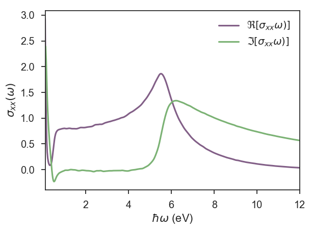
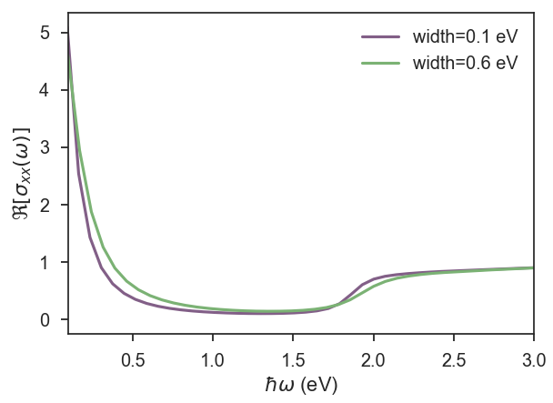
For systems sizes of N=1536 x 1536 unit cells and two different Gaussian widths, we show \(\Re [\sigma_{xx}(\omega)]\) for low frequencies (see Fig. 2). In both figures, one can clearly see the Drude's peak for \(\omega\rightarrow 0\) and the onset of interband transitions at \(\hbar \omega>2 E_F\) 2.
The complete Python script for this calculation can be found here.
-
Shengjun Yuan, Rafael Roldán, Hans De Raedt, Mikhail I. Katsnelson, Phys. Rev. B 84, 195418 (2011) ↩
-
T. Stauber, N. M. R. Peres, A. K. Geim, Phys. Rev. B 78, 085432 (2008) ↩
-
S. M. João et al, R. Soc. open sci. 7, 191809 (2020) ↩