1. Workflow
KITE has three different layers:
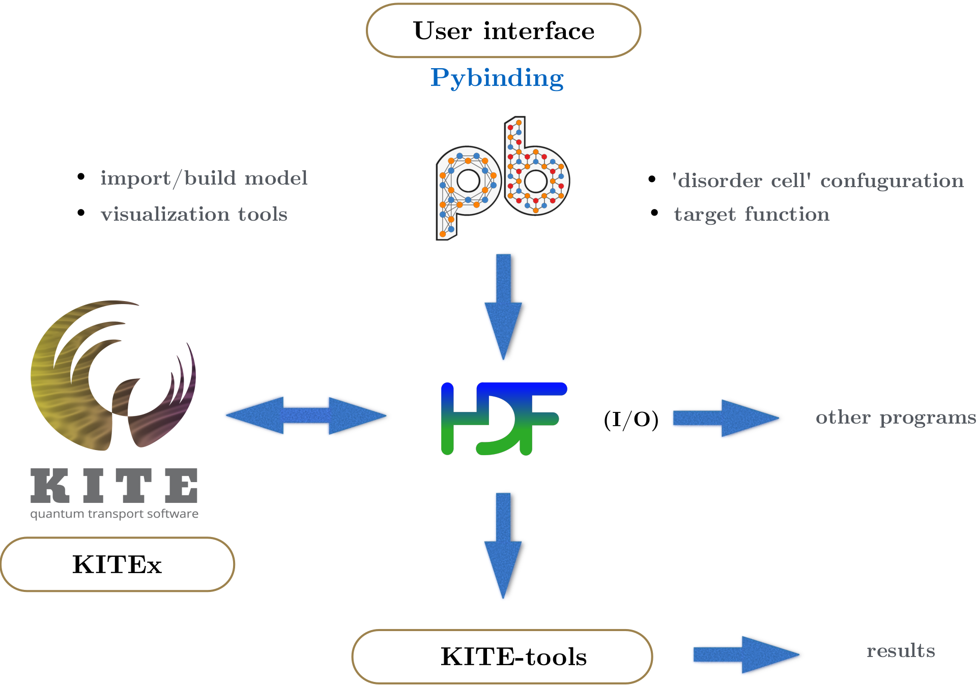
The tight-binding (TB) model is defined on a Python interface based on Pybinding. The TB parameterization benefits from a number of KITE-specific advanced features, including disorder patterns and magnetic-field modifications. The KITE model - which includes the desired target function calculations, such as the DoS - is exported to a HDF5-file, together with the calculation settings (i.e. system size, boundary conditions, parallelization options, etc.). This file is then given as an input to the main program (KITEx). The input and output for the main program are written to the same HDF5 file. The complete workflow is summarized in the figure below.
Steps
- Start by building a
pb.Latticethat describes a regular tight-binding model (Section 2) - Add optional terms to the TB Hamiltonian, including disorder patterns and a magnetic field (covered in Section 6 and 7)
- Specify the calculations settings (Section 3) and the desired target functions to be computed (Section 4)
- Export your KITE model to the HDF5 file and run KITEx (Section 4)
- Post-process the data using the post-processing tools KITE-tools and visualise the data (Section 5)
Tip
It is possible to use a simple python script for the whole workflow.